Introduction
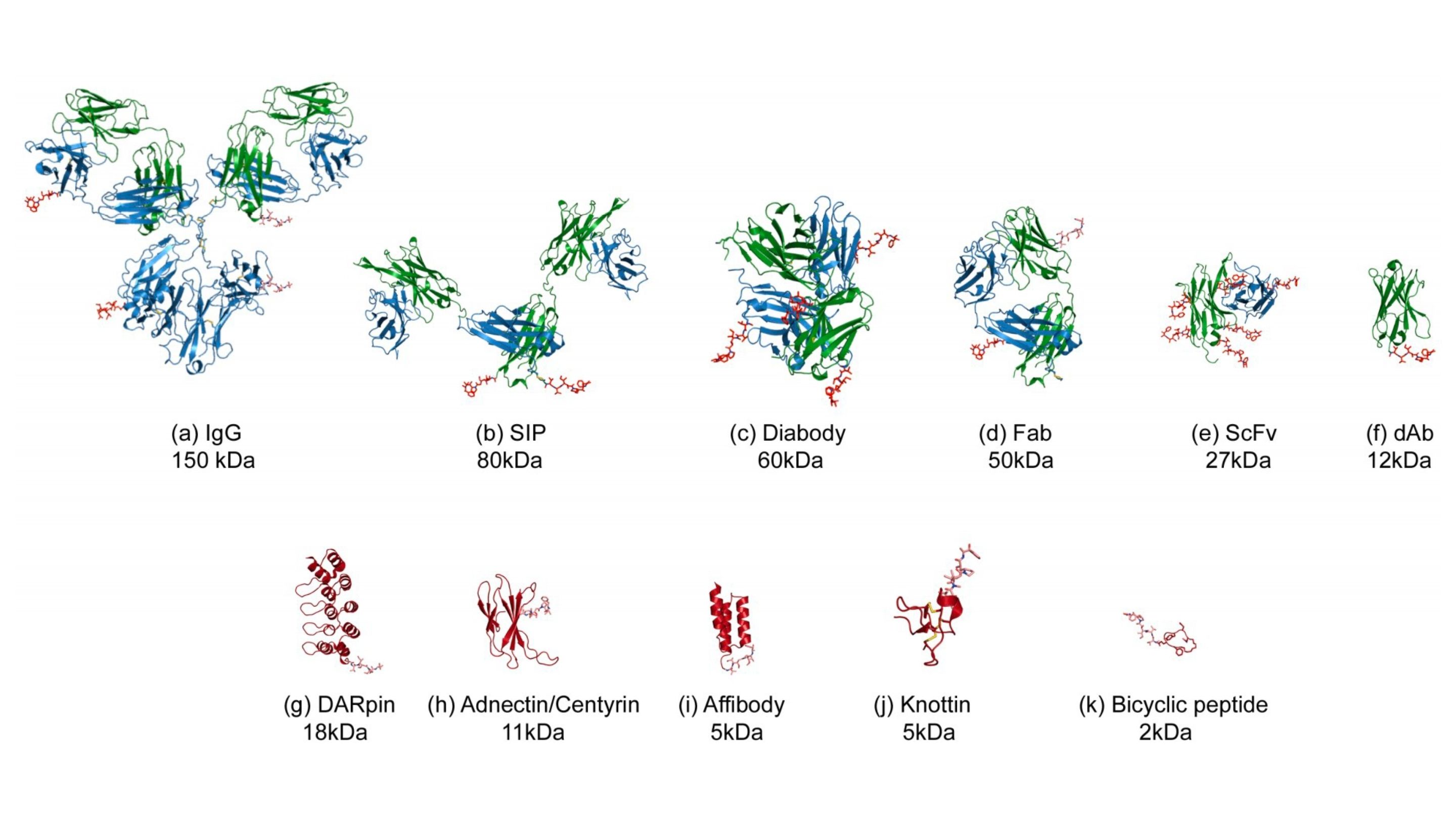
Biologic drugs are increasingly becoming important as therapeutics for treatment of various diseases, including cancer, infectious and inflammatory diseases. Classical antibody scaffolds and structures are being challenged by smaller but equally potent molecules which have several benefits over classical immunoglobulins.
Camelid antibodies have been shown to lack the light chain only carrying effector function on the heavy chain which have made them remarkably interesting from a therapeutic perspective. The variable domain itself separated from the constant region has been named nanobody. A thorough review of nanobodies and therapeutic relevance is beyond the scope of this application note but it nicely outlined in the review paper by Steeland et al.
Advanced bioinformatics and sequence analysis has become an integral part of antibody drug discovery and development and is being challenged by ever increasing amounts of sequence and functional data.
Pipe | bio offers an integrated, comprehensive yet easy to use cloud-based sequence analysis platform and advanced data repository which can easily be configured to cope with various annotation requirements for both antibodies and non-antibody scaffolds.
Biopanning, repertoire analysis, and immunization campaigns are all part of the toolbox to find valuable antibodies and other biologics and in this application note we show how we have used the Pipe | bio platform for analysis of high throughput (NGS) sequencing data of nanobodies (single domain antibodies) and how to find enriched clones in a biopanning experiment of Alpaca (Lama pacos), Miyazaki et al.
Here we reproduce key analysis components from the Miyazaki et al. paper within an hour in Pipe|bio software. In total we found 11 of the 12 clones identified in that paper. This blog post follows 6 steps:
- Merge of paired-end data
- Annotation
- Highlevel overview with charts
- Clustering on individual samples
- Multi-sample comparison
- Slice and dice the data
- Re-covering clones
- Alignments and further analyses
Data
For this application note, we have retrieved two datasets from the European Nucleotide Archive.
- Bioproject: https://www.ebi.ac.uk/ena/browser/view/PRJDB2382
- Paper: doi: 10.1093/jb/mvv038
This is the dataset used throughout the application note. We also used data deposited in Genbank with accession numbers AB926001-11 for validation.
- Total read count: 1,372,580
- Bioproject: https://www.ebi.ac.uk/ena/browser/view/PRJNA321369
- Paper: doi: 10.1371/journal.pone.0161801
This dataset is used as an illustration of “historical” sequences to represent internal company sequences, patent sequences, public repertoire data etc. This dataset has been analysed and put into the sequence store but is otherwise not used in the application note.
- Total read count: 4,851,448
Scaffold configuration
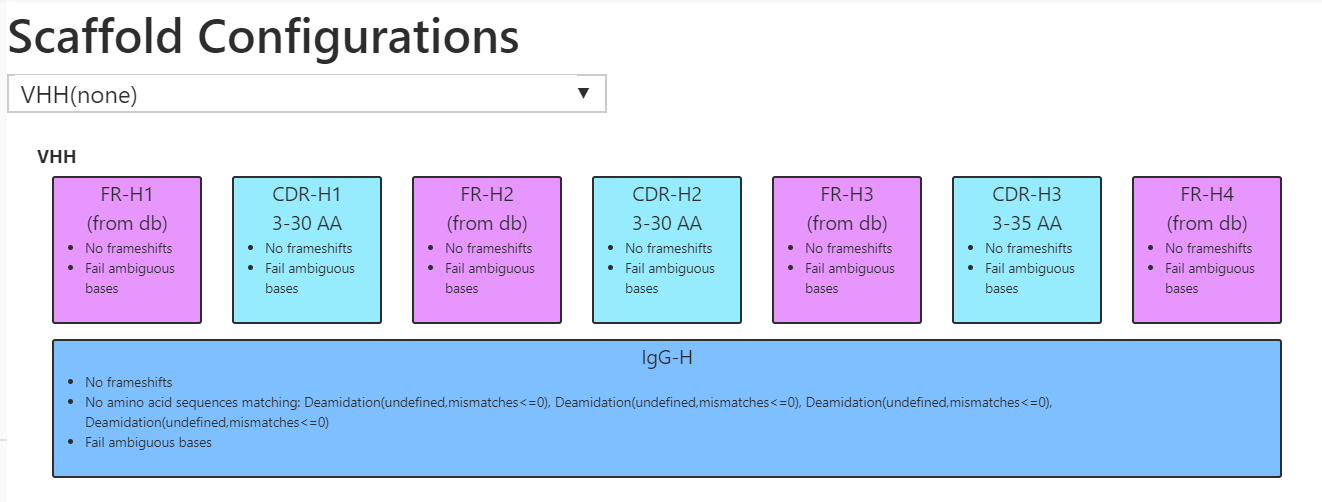
Before running the annotation pipeline, there is a one-time configuration of the required scaffold. Examples of a scaffold can be IgG, ScFV, nanobody, non-antibody etc. and below we show a simplified example of a nanobody scaffold. As part of the scaffold configuration it is possible to specify any liabilities, disallowed frameshifts, stop codons, glycosylation sites etc. and how this should be reported in a tabular output.
Multiple scaffolds can be configured allowing for different configurations enabling teams to work on different molecules in the same platform.
Analysis pipeline
The PipeBio platform is very flexible and here we perform a relatively simple workflow.
- Import sequences
- Merge paired-end sequences
- Annotate sequences according to scaffold configuration
- Plot various findings
- Cluster regions of interest
- Find enriched clones
We also look up common sequences in our database of “historical” sequences.
Merging paired-end data
The data was imported by drag and drop into the platform and sequence quality was visually inspected visually with a quality score diagram.
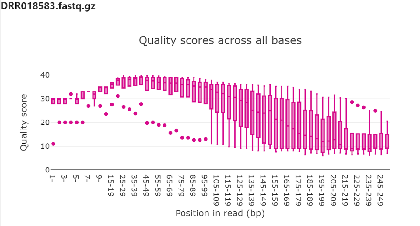
It is obvious that the quality of the raw data is questionable and thus will need to be trimmed to remove poor quality to get reasonable accuracy of the downstream annotation pipelines.
The raw fastq files are in the (rarely used) interleaved format, thus quality trim was carried out with command line versions Cutadapt (Martin et al.) to trim bases below Q20.
Basic statistics
Here are some basic statistics of the two individual samples before and after the biopanning.
It is worth mentioning that we have used different trimming options than described in the paper which in our case give a higher number of sequences which are correctly annotated than compared to the paper.
Annotation results
The output of the annotation pipeline is a result document which shows detailed tabular information aligned with the sequences in a graphical view. This enables the user to performs advanced filters and interpretation of the tabular data while having the visual representation of the annotated sequence The annotation results are accompanied with a graph showing breakdown of identified liabilities and other problems as specified in the scaffold. See table 1.
A high proportion (~83%) of the merged reads can be fully annotated (incl. FR1 – FR4) as seen from the pie chart in figure 4.
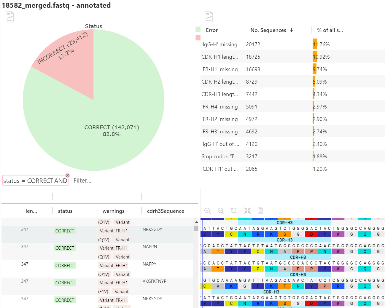
The pie chart in the upper pane show an overall summary of the annotation rate and detailed statistics on errors and liabilities as specified in the scaffold. The lower pane shows a detailed tabular breakdown of the annotated sequences including the actual sequence. This view can be configured to the users liking.
Charts
It is possible to plot different charts to support the analysis and workflow. These can be made per region or the full-length sequence. All charts and pipelines support filtered input. All charts are interactive, thus clicking on the chart will apply a filter in the result table. For example, clicking the “CORRECT” section of the overall summary pie chart will filter so only correctly annotated sequences are shown. See figure 4.
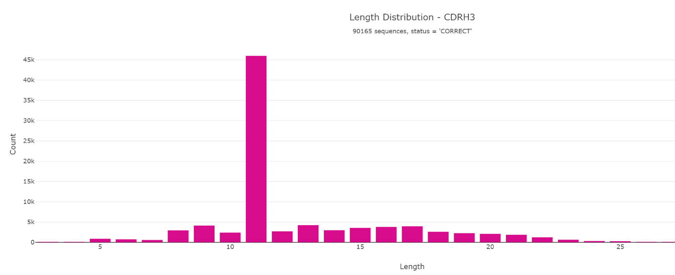
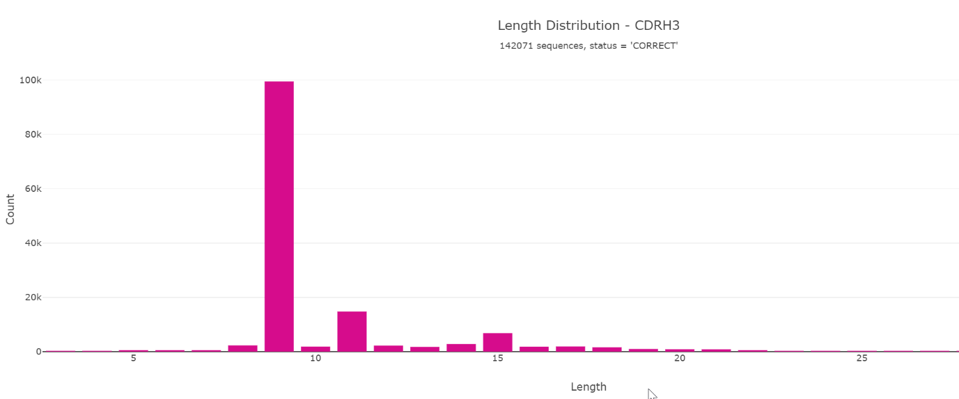
Looking at the amino acid sequence length of CDR-H3 of the Miyazaki et al. paper reveals an unusual distribution.
Various other charts are available which can help to interpret and identify interesting characteristics of the nanobodies.
- Codon usage
- Length distribution
- Sequence logo
- Amino acid heatmap
- And more…
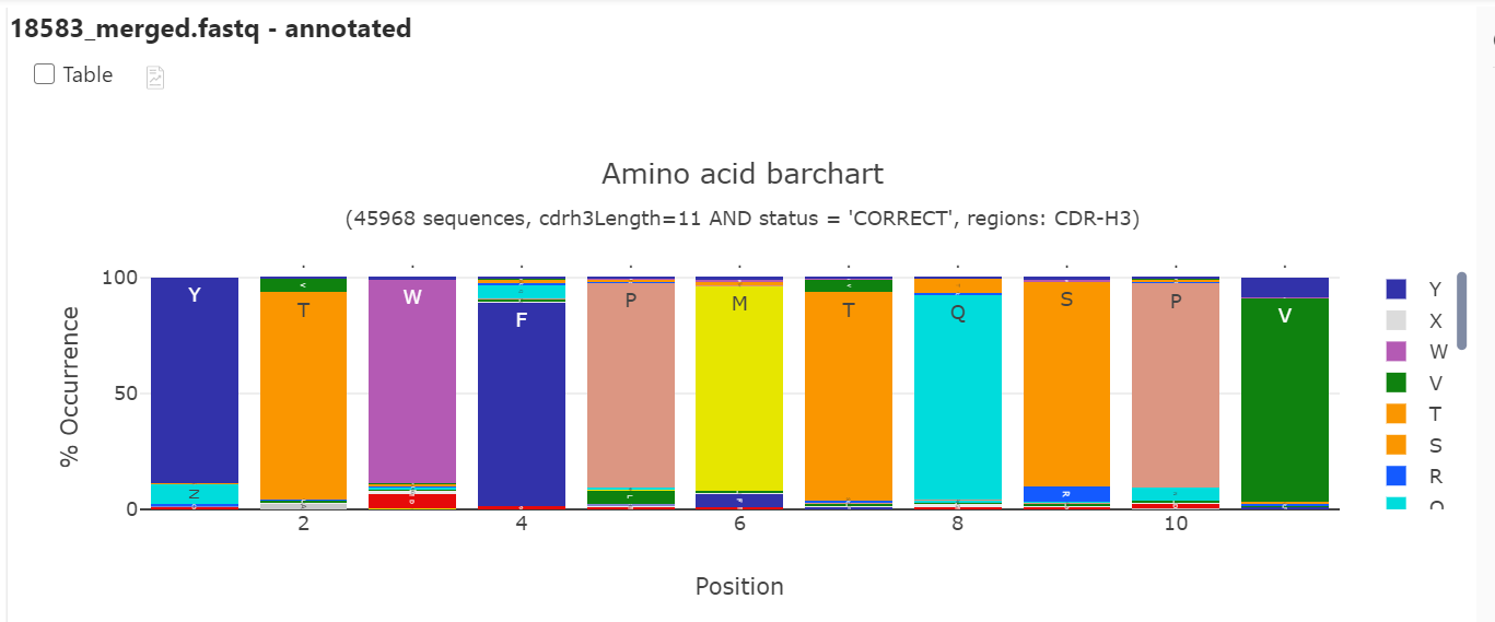
The length distribution looks very biased and by making a stacked bar chart it seems likely that only one sequence dominates the library. This can also be confirmed by clustering where we identified 41804 identical CDR-H3 (YTWFPMTQSPV) sequences before panning. Furthermore, this is described in the original research paper.
Clustering on individual samples
To investigate sequence diversity we performed clustering on the two samples from before and after biopanning. This enables us to see how many unique sequences contribute to each subcluster and can also be used to look into the skew of the data in figure 5.
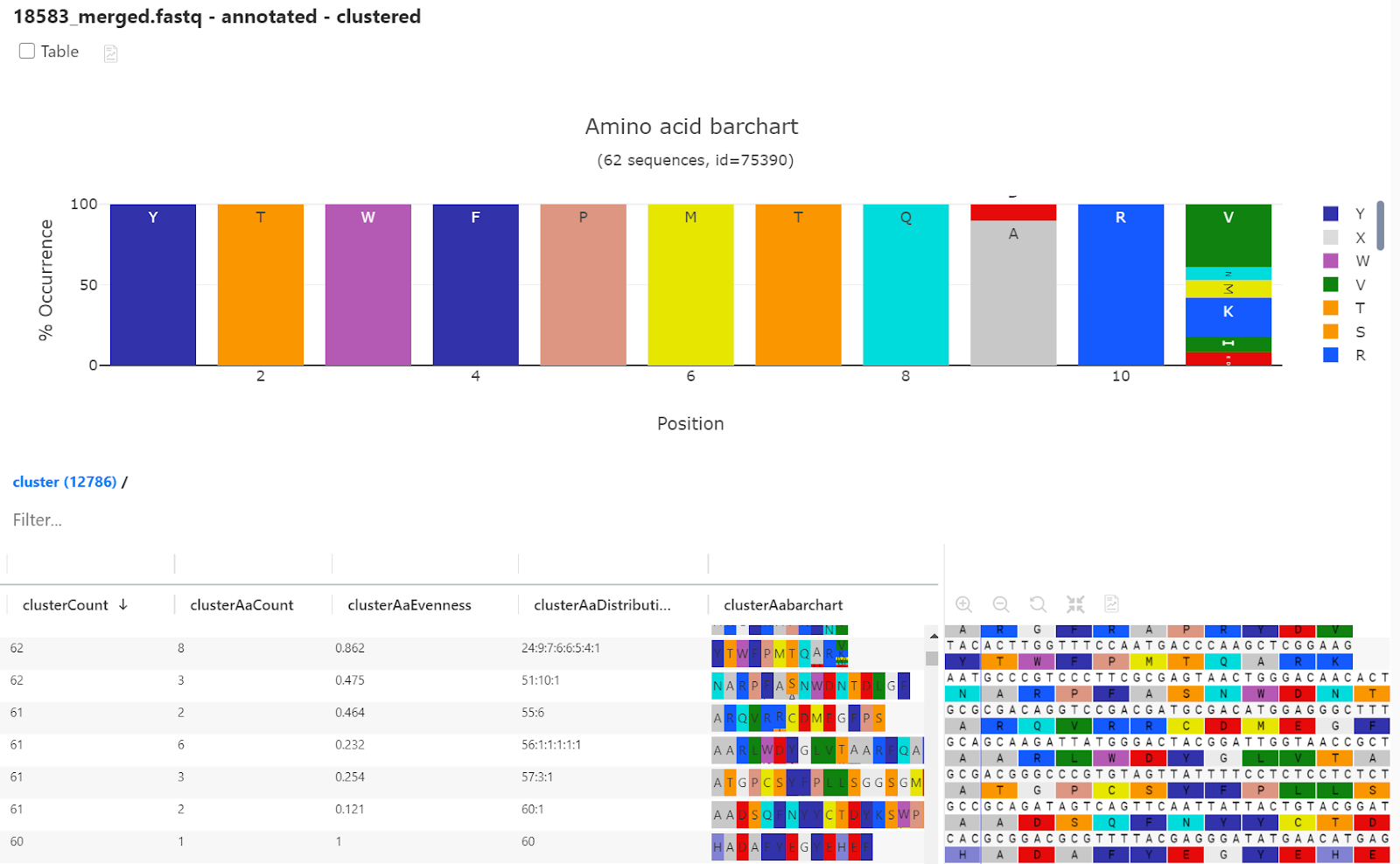
In Fig. 8, an inline bar-chart is used to quickly identify variability of the subcluster. A larger barchart in the upper half of the screenshot show variability in position 9 and 11 of the first subcluster.
Distribution and counts of individual sequences within a subcluster are represented as numerical values in the result table. Evenness is a measure of the distributions of sequences in a subcluster. If there is an equal distribution of unique sequences in a subcluster the evenness score is 1. A high over-representation of one unique sequence in a cluster will result in a very low evenness score. For additional information see docs.pipebio.com
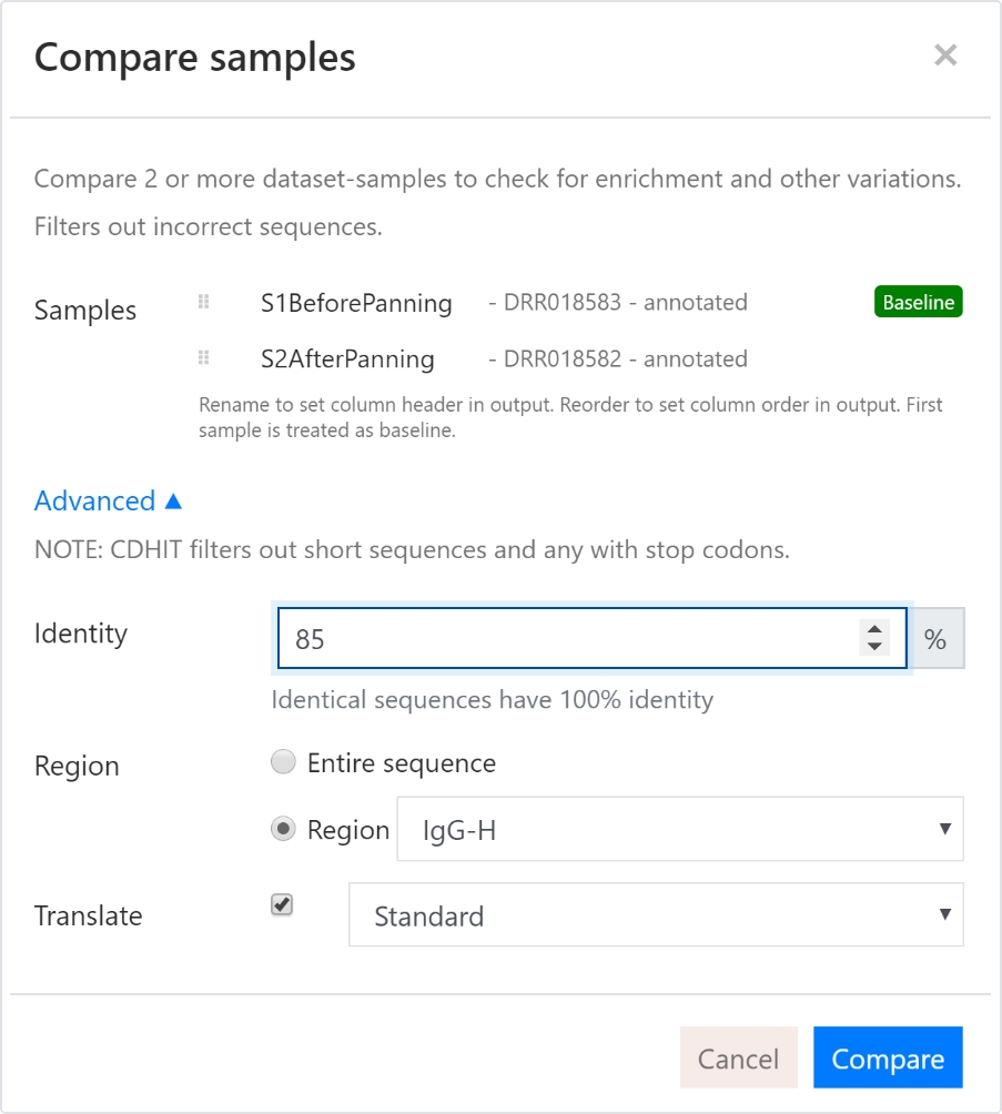
Multi-sample comparison
There are many use cases for comparison of NGS samples. As examples, it is interesting to see clonal expansion during selection rounds, affinity maturations, compare patient cohorts to a control group, or other types of enrichment projects. This is very easy to do in the Pipe | bio platform.
Here we compare the two samples from before, one before panning and one after panning.
When looking at the result it can sometimes be desirable to get rid of low count clusters which may be statistically irrelevant. These singleton clusters can potentially be sequencing errors and will require additional interpretation of the raw sequence reads. In this application note we keep all the data and will later explore if there are singleton clusters before panning which could be interesting to look at due to high expression in the latter sample.
Slice and dice the data
Here we show different effects of filtering the data. There may be valuable information lost if singleton clusters are removed prior to performing the analysis, thus we choose to keep those in this experiment. In some situations, it may be relevant to get rid of low count sequences in the result as these may be sequencing errors.
Although this a small dataset we further want to reduce it down to a tangible number sequence to cherry-pick for additional analyses and functional assays.
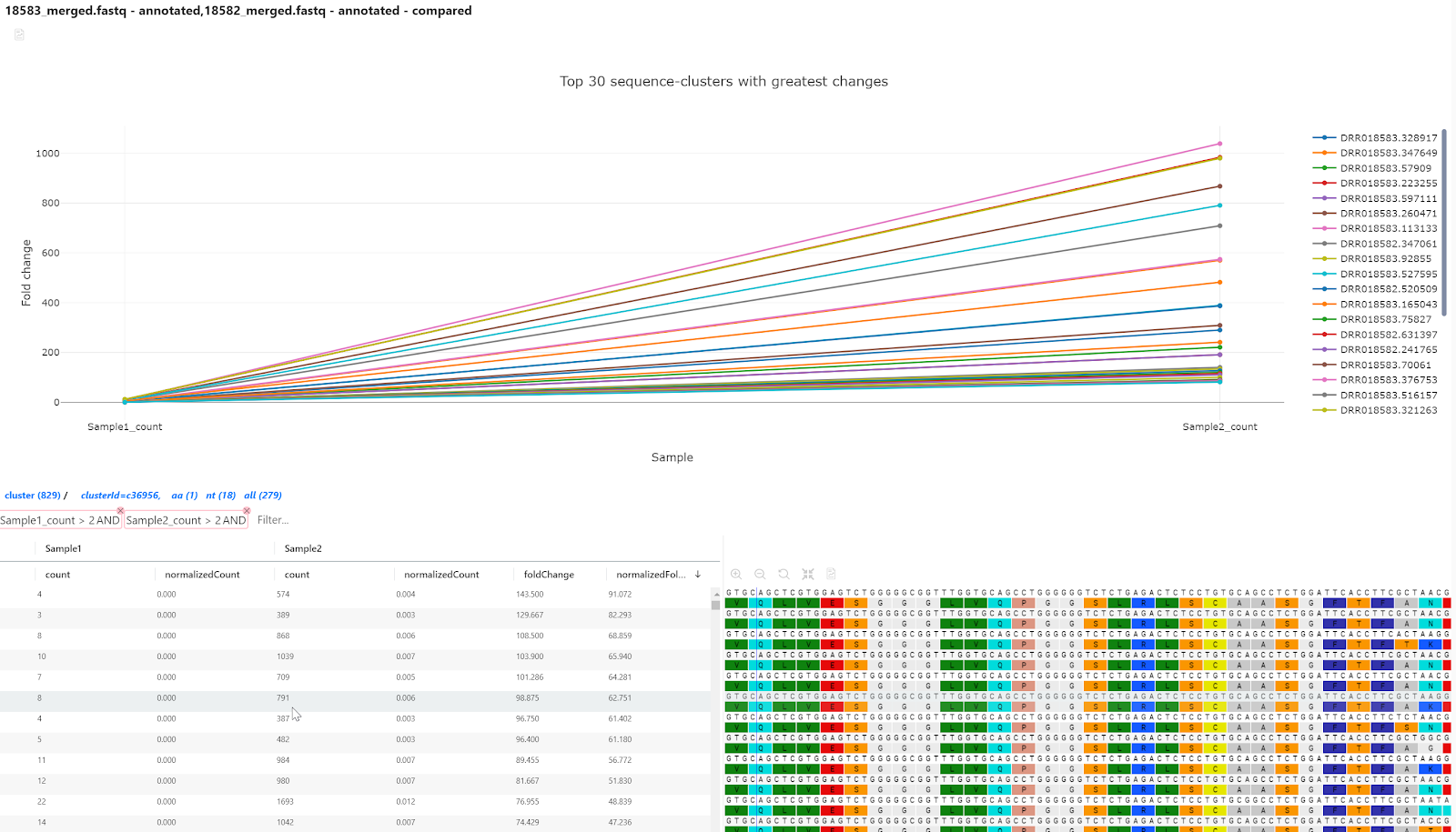
Below are some examples of filters find potential great candidates which are enriched. The built-in autocomplete for filters are useful as the column names are influences on how we have named the samples in the Compare samples dialog. See figure 9.
When doing panning experiments, it is difficult to know if a given antibody sequence is containing a sequence error or if it is a real sequence due to a true somatic hypermutation. As first example, we chose to filter out all low frequent clones to not pollute our results. We simply remove low count sequences from both samples by using the filter below.
- Filter1: S1BeforePanning_count>2 AND S2AfterPanning_count>2
If we furthermore only want to look at sequences which are enriched more than 10 fold we add this to our filter. We have chosen the normalized fold change to account for differences in sample size.
- Filter2: S1BeforePanning_count>2 AND S2AfterPanning_count>2 AND normalizedFoldChange>10
Finding antibodies on the rise! Sometimes it is interesting to see if no clones were present in the beginning and is being expressed as part of the selection pressure. Thus, we want to filter for sequences which are present in very low numbers before panning and in large number after panning. On top of this we apply a filter for the normalized foldchange.
- Filter3: S1BeforePanning_count<3 AND S2AfterPanning_count>2 AND normalizedFoldChange>10
These findings are summarized in the table below. Included is clustering and filtering only on CDR-H3 to show differences in clustering in different length regions.
Removing very low count sequences/clones reduces the number of sequences significantly. For full length nanobody enrichment we find 54 sequences which have 10 fold enrichment when normalized to sample size.
Recovering clones
From the Miyazaki et al. paper it is interesting to see if we are able, from an informatics perspective, to recover the clones they have identified as interesting binders.
Miyazaki et al. selected 13 clones using ELISA which are listed in the table below. We have identified 11 of those in our list of 54 mostly enriched clones. We do not have sequence data for N14 as this clone was not deposited in GenBank and N7 was filtered out due absence in sample1.
It would be very interesting to have functional data on all 54 enriched sequences.
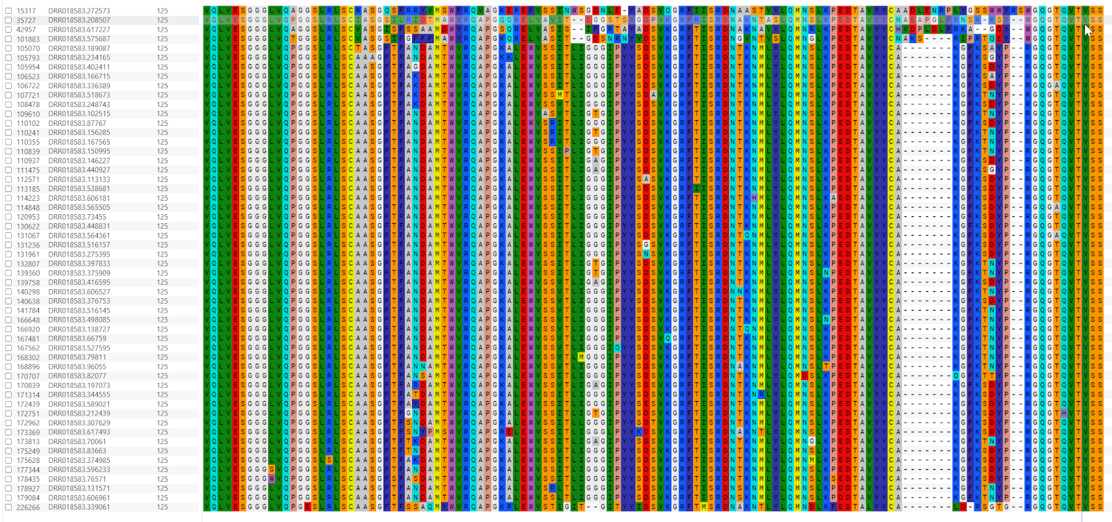
Alignments and further analyses
To visually look at the sequences, the 54 sequences were extracted and aligned for further inspection.
Sequence Store
An important step in drug discovery and development is investigating whether the sequences of interest have been seen in public repertoires or patent databases.
We have analyzed the 4,851,448 sequence from PRJNA321369 and deposited these in the sequence store and use those sequences as an example of historical sequences or public domain data.
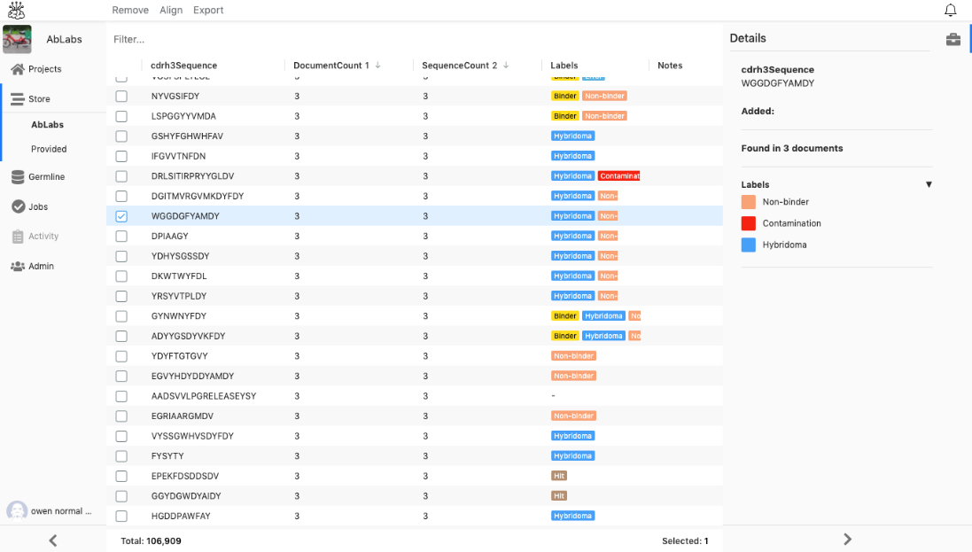
None of the 54 interesting and most enriched clones were found in the store of the PRJNA321369 data.
Conclusion
With the sequence data available in the Miyazaki et al. paper we were informatically able to recover 11 out of 12 clones (one sequence is not present). All the analysis took only a less than one hour from import of merged data to export of cherry-picked list of 54 clones. It would be very interesting to see functional assays performed on the remaining 42 clones we identified as being highly enriched but this information is not available in the paper.
We have also identified 81 sequence which was expressed in very low levels before panning but highly abundant after panning. These could also be interesting to investigate further.
.jpg)